Equitable Valuation of Pretax Assets

Too often, neither financial analysts nor attorneys understand all the complexities with valuation and division of pretax assets. Misunderstandings cost clients tens or even hundreds of thousands of dollars. These assets often represent some of the most significant components of marital wealth, but their equitable valuation is complicated because they offer limited liquidity and will be subject to taxation upon distribution. This study offers an in-depth look at how to properly value retirement accounts like IRAs and 401k accounts.

At times, retirement accounts are not divided 50/50 between spouses and may be traded for other valuable assets like the family home. While most states’ statutes include provision to account for tax effects when valuing pretax assets, case law commonly places burden on a spouse to present justification that deferred taxes affect equity. This post explores the underlying concepts to help justify and quantify an equity assertion.

Background:  Methods of Division

Pretax and tax-free retirement assets face different tax consequences than taxed assets. The division of retirement assets for divorce typically involves using one of three methods:

• Deferred division
• Current equal division
• Present-value offset

Each approach offers a different way to calculate and allocate the marital portion of the asset. The choice of method often depends on the preferences of the divorcing spouses and the specific nature of the asset.

Deferred Division Method

The deferred division method, also called the “wait-and-see” approach, allows the non-employee spouse to receive a share of the asset when the employee spouse retires or begins receiving payments. Under this method, the asset remains intact until it is time for distribution and the non-employee spouse receives a percentage of each payment based on the marital portion of the asset. This approach is commonly chosen for its simplicity, as it avoids the need to estimate the pension’s future value. This method also better ensures equity because both spouses experience the same uncertainty as they await division of the asset.

This method requires a Qualified Domestic Relations Order (QDRO), Court Order Acceptable for Processing (COAP), or similar court order to be prepared and submitted to the plan administrator, directing them to pay the non-employee spouse a stated share of the retirement asset upon the employee spouse’s retirement.

Current Equal Division Method

The current equal division method may offer the easiest means of calculation and removes all speculation of future value by dividing and distributing the marital equity close to the date of settlement. After each spouse receives their equitable distribution at settlement, each spouse can be accountable independently for whether and how to invest their equity. This method is predicated on the asset having sufficient liquidity to be divided and distributed between the two spouses at the time of divorce. More ambiguous assets such as pensions that have more speculative value until retirement may not be candidates for this method.

This method may require a QDRO or similar court order for assets like a 401(k). However, the division of an IRA is typically handled as a “transfer incident to divorce”. A spouse should consult with an attorney and/or a tax accountant to ensure withdrawals and transfers occur without tax penalty to either spouse.

Present-Value Offset Method

In this method, the asset is assigned a present-day value, allowing the asset-retaining spouse to buy out the non-retaining spouse’s marital share while keeping the asset intact and pretax. This method requires a valuation of the asset based on factors like the account’s growth rate, expected withdrawal or annuity age, and life expectancy.

This method introduces the flexibility for one spouse to offer a quid pro quo compensation to retain the full value of the retirement asset. For example, the spouse retaining the retirement asset could compensate the other spouse with a lump sum from other marital assets, such as the family home or savings accounts. This quid pro quo compensation can involve complicated analytics and is the focus of this study.

Common Mistakes

A lot of confusion stems from misunderstandings of tax deductions (eliminating tax) and tax deferral (paying tax at a future date).  Think of a pretax asset as including two parts:  a Base and a Tax as shown in Figure 1.

Figure 1:  Current Tax Burden for Current Asset Value

If the asset were distributed and taxed today, the Base would exist after the Tax was paid to the taxing authorities. For some types of retirement accounts like traditional IRAs and 401ks, the tax gets deferred until withdrawals are made in retirement. The most common mistakes are:

1. Ignoring the difference in value between pretax and after-tax equity:  A dollar of pretax equity will incur a tax liability that a dollar of after-tax equity will not.
2. Assuming immediate withdrawal:  The pretax asset is valued as if it would be taxed immediately. Subtracting an immediate tax cost from a pretax asset ignores the effects of market growth and deferred taxes on pretax versus non-pretax assets.
3. Applying an incorrect tax rate:  The asset will get taxed at the marginal tax rate at the time of withdrawal for the owning spouse based on the taxable income and tax brackets at the time of withdrawal. Errors include using average effective tax rates, tax rates based on joint marital income levels, and tax rates based on pre-divorce marital status.
4. Incorrectly calculating present value:  When applying the Present-Value Offset Method, the present value of both the base plus deferred tax needs to be reflected. Many analysts mistakenly forget that the deferred tax will accumulate growth, and much of that growth will remain after tax.
5. Ignoring the present value of cash:  The respective present values of two assets offer a fair comparison, but some analysts mistakenly assume that the present value of cash equals the current value of cash. Doing so ignores the growth opportunities and tax burdens over time of investing cash.

We will quantify these common errors later in this study.

Foundation for Equitable Valuation:  Calculating Present Values

Two primary types of tax-affected retirement accounts exist:  a fully deferred tax account such as a 401(k) or traditional IRA and a tax-free account such as a Roth IRA. As will be shown, for these types of retirement accounts and for after-tax accounts, present values differ. The general approach to calculating present value can be seen in Figure 2. However, different types of accounts may exclude value for parts of this figure, may experience different growth rates in phase 2, and/or incur different tax rates in phase 3.

Figure 2:  Four Phases of Progression for Present Value of a Pretax Asset

This figure shows the four phases to calculate present value:

• Phase 1:  At present, the asset’s face value includes a base value and a tax that would be paid if the asset were withdrawn at this time (excluding any early withdrawal penalties).
• Phase 2:  Both the base and the deferred tax value experience market growth until the asset is withdrawn from the pretax account.
• Phase 3:  The deferred tax is paid for tax liabilities based on the current pretax fact value (Base + Deferred Tax). The market growth for both Base and Deferred Tax value is taxed.
• Phase 4:  The after-tax value (Base plus taxed growth) gets discounted to present value.

Variables for Present Value Algorithms

To derive our algorithms for valuation, we reconstitute Figure 2 with corresponding variables in Figure 3.

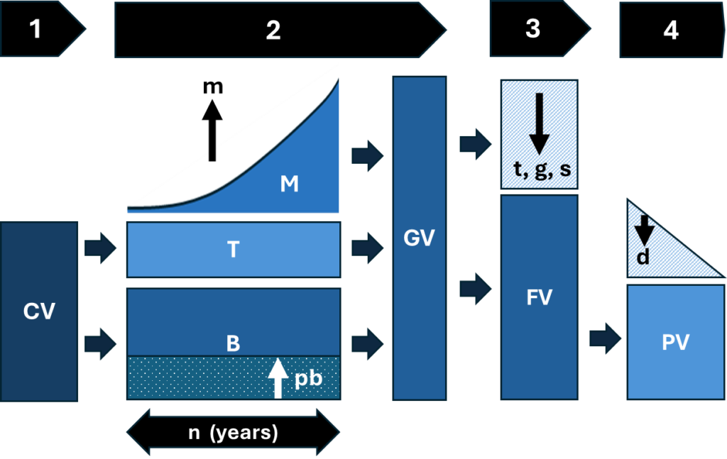
Figure 3:  Variable Representation Across Phases of Present Value

To summarize our variables:

• Current pretax face value (CV):  The face value of the asset at the date of valuation
• Base value (B):  The value of the CV that would remain after taxes were paid
• Principal basis (pb): The principal (or cost) basis against which capital gains are calculated
• Tax value (T):  The value of the tax burden of the CV
• Market growth (M):  The increase in value of the CV of the asset resulting from market forces such as interest or asset appreciation from the onset (e.g., date of settlement) until date of distribution of the asset
• Market growth rate (m):  The compounded annual growth rate for the CV of an asset from the current date until date of distribution
• Deferral timespan (n):  The number of years the asset will delay distribution (remain pretax)
• Grown value (GV):  The sum of the CV plus the market growth
• Future value (FV):  The after-tax value of an appreciated asset (i.e., GV)
• Federal tax rate (t):  The estimated marginal federal tax rate that will be applied to the distribution of the pretax asset or to interest of a taxed asset
• Capital gains rate (g):  The estimated rate of federal capital gain taxes that will be paid because a post-tax asset increased in market value
• State tax rate (s):  The estimated marginal state tax rate that will be applied to the distribution of the pretax asset or to interest of a taxed asset
• Present value (PV):  The value of an asset that represents is CV plus the and the discounted value (cost of money) of any cash flow or market growth until the end of the asset’s life
• Discount rate (d):  The rate of return used to reflect the cost of money through the life of an asset (many times, Treasury Bills with a similar lifespan are used)
• Equivalency rate (e):  The comparison between the present value of an post tax asset to a pretax asset, signifying how many dollars post tax currently equals the a dollar of present value for a pretax asset

Present Value of a Fully Deferred Tax Retirement Account

In a fully deferred tax account (like a 401k), the asset is taxed upon withdrawal after the initial (current) value of the asset has experienced market growth. The withdrawal incurs income tax at the owner’s marginal tax rate, and that post-taxed value gets discounted to present value.

The general equation is:

GV   =   CV * (1+m)^n

FV   =   GV * (1-t)    =    CV * ((1+m)^n) * (1-t-s)

PV   =   FV / (1+d)^n   =   CV * ((1+m)^n) * (1-t-s)) / (1+d)^n  

Present Value of a Tax-Free Retirement Account

In a tax-free account (like a Roth IRA), the asset contributions were post-tax, so the current value equals the base value (i.e., CV = B, and all the light blue shaded tax deferral in Figure 2 are excluded). The growth on the remaining Base is not taxed when the asset is distributed or liquidated.

With similar assumptions, the general equation is:

GV   =   CV * (1+m)^n

FV   =   GV    =    CV * (1+m)^n

PV   =   FV / (1+d)^n   =   CV * ((1+m)^n) / (1+d)^n  

A dollar in a fully deferred tax account should be worth less than a dollar in a growth-deferred tax account.

Present Value of a Taxed Account

A taxed account holds assets that were acquired with taxed equity, so again CV = B. However, if the after-tax contributions to this asset (pb) have totaled less than CV, capital gains taxes could be pent up (such as for equities or real estate) and would need to be reflected in PV. As the taxed base grows, the growth is subject to either annual income tax (such as for interest payments) or additional upon-distribution capital gains taxes.

The federal government sets federal capital gains rates and regulations. However, most states treat capital gains as ‘ordinary income’. While most states that have an income tax treat capital gains the same as regular income, a significant minority of states either have no state income tax, provide preferential rates for long-term gains, or offer deductions/exclusions. Understand your state’s tax laws and adapt the following equation accordingly.

The general equation for an asset whose capital gains are taxed only upon withdrawal (such as for stocks) is:

GV   =   CV * (1+m)^n

FV   =   GV – (GV-pb)*(g+s)

       =   CV * (1+m)^n – (CV * (1+m)^n – pb)*(g+s)

       =   CV * ((1+m)^n) – CV*((1+m)^n)*(g+s) + pb*(g+s)

       =   CV * ((1+m)^n) * (1–g-s) + pb*(g+s)

PV   =   FV / (1+d)^n   =   (CV * ((1+m)^n) * (1–g-s) + pb*(g+s)) / (1+d)^n  

The present value when the tax on asset growth occurs annually (such as for interest-bearing accounts) is:

GV   =   CV * (1+m*(1-t-s))^n

FV   =   GV    =    CV * (1+m*(1-t-s))^n

PV   =   FV / (1+d)^n   =   CV * ((1+m*(1-t-s))^n) / (1+d)^n  

Calculating  Equivalency

A key need for this analysis involves equitably compensating the spouse that does not receive the tax deferred account in settlement. Because any type of account can be used to compensate the other spouse, a ‘cash equivalent’ method typically is used. All assets are normalized compared to the present value of after-tax cash. Otherwise, the following calculations would need to be expanded for all permutations of every type of asset.

Two assumptions commonly offer the fairest comparison. Exceptions can be treated on a case-by-case basis.

1. The present value of the taxed and pretax assets should reflect the same lifespan. In rare exceptions, the timeframe (n) can be replaced with n_taxed and either n_untaxed or n_tax-free. 
2. Present value normally reflects optimizing opportunity cost, so both assets should be invested to achieve their maximum present value. Depending on factors such as risk tolerance, equivalency typically assumes that after-tax cash would be invested in some combination of interest and/or equity bearing financial instruments. In our following analysis, we assume both assets would invest in stocks. Both m_taxed and either m_untaxed or m_tax-free would have equal rates.

The common derivation for compensating retirement accounts with after-tax cash are: 

For buying out a fully deferred tax retirement account:

PV_taxed   =   PV_untaxed

(CV_taxed * ((1+ m_taxed)^n * (1–g-s) + pb*(g+s)) / (1+d)^n   =   CV_untaxed * ((1+m_untaxed)^n) * (1-t-s) / (1+d)^n  

CV_taxed * ((1+ m_taxed)^n * (1–g-s) + pb*(g+s)   =   CV_untaxed * ((1+m_untaxed)^n) * (1-t-s) 

CV_taxed  =   (CV_untaxed * ((1+m_untaxed)^n * (1-t-s))  – pb*(g+s)) /  ((1+ m_taxed)^n) * (1–g-s)

For buying out a tax-free retirement account:

PV_taxed   =   PV_tax-free

(CV_taxed * ((1+ m_taxed)^n * (1–g-s) + pb*(g+s)) / (1+d)^n    =   CV_tax-free * ((1+ m_tax-free)^n) / (1+d)^n  

CV_taxed * ((1+ m_taxed)^n * (1–g-s) + pb*(g+s)   =   CV_tax-free * ((1+ m_tax-free)^n)  

CV_taxed   =   (CV_tax-free * ((1+ m_tax-free)^n)  –  pb*(g+s)) /   ((1+ m_taxed)^n) * (1–g-s)

The complexity of these algorithms emphasizes the effect of how different types of assets are taxed. If we ignored the ‘Common Mistakes’ listed earlier, we also would ignore many of these variables and fool ourselves to believing the equivalencies are simpler. For example, if we ignored future federal and state taxes on the capital gains of investments from equivalent cash and assumed equal growth rates in the investments from both accounts, our equivalencies would simplify to more familiar (but likely more inequitable) algorithms:

• CV_taxed  =   CV_untaxed * (1-t-s) 
• CV_taxed   =   CV_tax-free

Uncertainty with Methodology

Estimates are estimates. By definition, they are inexact. However, a good estimate can minimize uncertainty and offer the best means to quantify an item.

Some contributors to uncertainty may include:

• Tax rates:  The future tax code may experience changes such as tax brackets and tax rates. Current rates and brackets typically offer the most accurate estimate of the future; however, the status of pending changes to tax law may be warranted otherwise.
• Income levels:  The taxable income for the owning spouse after n years may vary from estimates and pertain to a different-than-estimated marginal tax bracket. Analysis to forecast the spouse’s income after n years could improve uncertainty.
• Filing status:  The relationship status for the owning spouse after n years may vary and may pertain to a different filing status that may incur a different marginal tax rate. The “single” filing status is a default consideration, but an assessment of the spouse’s personality and situation may suggest a better filing status.
• Year of withdrawal(s):  Distributions can occur at different years and distributions can occur at multiple years. A more detailed assessment of the owning spouse’s retirement and income plans may yield a more accurate representation of withdrawal schedule that may yield a more accurate PV for the pretaxed asset. If we can assume that the market growth rate of the pretaxed asset is the same as that available to the post-tax assets that will compensate the other spouse, the year of withdrawal will not affect the equivalency calculation.
• Market growth rate:   Actual growth rates vary for different types of assets and even for different assets in the same asset type. For maximum accuracy, consider the current type of assets but also consider whether the type of assets are likely to change. For example, many investors start migrating from higher risk equities to lower risk interest-bearing assets as they progress closer to retirement age. If we can assume that the market growth rate of the pretaxed asset is the same as that available to the other spouse’s post-tax assets, the market growth rate will not affect the equivalency calculation.
• Market growth rate:   Actual growth for assets such as mutual funds can change by the second, and growth volatility traditionally has varied within a standard deviation of 15% for stocks and 5% for interest accounts. If pretax asset distributions are expected to occur within a short time horizon, a more accurate growth rate may be based on average historical rates from a shorter recent number of years.
• Taxing taxed investments:  Estimating tax effects can be complicated. Some hybrid accounts include both annually taxable interest and dividends and upon-withdrawal capital gains. And mutual funds commonly incur nominal capital gains each year as underlying stocks are bought and sold.

Exceptions Cases

Two primary exceptions exist, and each has different considerations.

Exception 1:  Reconciling other types of assets

As mentioned before, asset types other than after-tax cash can be used as compensation to the spouse that does not retain the retirement account. Awarding the family home to one spouse and the retirement accounts to the other is a common settlement approach.

In all cases where one asset is traded for another asset, the present values of both assets should to be equal to be equitable. In cases where assets that are not easily divisible do not have equal present values, the present value of other more easily divisible assets can be integrated into the equity calculations. This for example could involve adjusting how cash from bank accounts get divided in separation.

Exception 2:  Possibility of multiple or delayed distributions

This study assumed a lifespan of n years, for which n normally reflects the timespan until the account holder retires. In reality, many retirement accounts require multiple years for an account holder to delete. In some cases, they do not start withdrawing from retirement accounts for years until other non-retirement accounts are depleted. These diversions normally have little consequence on the results of equity analysis.

Figure 4 reflects a $100,000 retirement account invested in an S&P 500 index fund). This figure plots the after-tax cash current value equivalence for a fully deferred retirement account distributed totally in a single year upon retirement. Retirement could occur anytime between 1 and 30 years. As the plot shows, the equivalent after-tax cash value of the account varies little after about ten years, so trying to resolve exactly when a retirement that will occur more than decade away adds little value to an estimate.

Figure 4:  Change in Cash Equivalent Value Based on Year of Distribution

More specifically, the max error in Figure 5 calculates the error if a settlement assumes a full distribution after 20 years but the full distribution occurs any time between 1 and 30 years. The error is exceptionally small (less than 5%) unless the account withdrawal occurs more than 8 years prematurely, which rarely happens because early withdrawal penalties discourage early withdrawals.

The nominal error in Figure 5 shows the effect if the retirement account distributions are divided annually between year 20 and any time between year 1 and 30. The error from disregarding a spread distribution schedule is even more exceptionally small, especially for accounts whose distributions occur within a +/- 15 year span. If a person spread withdrawals across up to 10 years after retiring in year 20, the error should be within 2%.

Figure 5:  Error From Assuming All Account Distributions Occur in Year 20

In conclusion, retirement accounts estimated to be distributed after 12 years (or possibly after 6 years) chance little error regardless of how much later they begin distributions and for how many years after initiation the distributions are spread.

Quantifying Common Mistakes

We will focus on determining equivalency for a fully deferred tax retirement account. The correct calculation of equivalency can be shown in the following example. Spouse #1 owns a $100,000 retirement account.  To minimize the opportunity cost disparity between taxed and untaxed accounts, we will assume that the taxed accounts include a mutual fund that performs growth like the tax-deferred account (i.e., m_untaxed = m_taxed).

Here are the example factors:

• CV_untaxed:  $100,000
• pb: $100,000 (assumes capital gains will incur only on growth after divorce)
• n:  20 years until total withdrawal occurs at the onset of retirement
• m:  10%, based on the average S&P growth rate over the last 30 years
• t:  32% federal marginal income tax rate
• s:  6% state marginal income tax rate
• The asset owner earns too much income to receive any related state tax deductions related to pretax distributions
• g:  20% for long term federal capital gains rate

Correctly Estimated Equivalency

In our example the value of a taxed asset to compensate spouse #2 would be:

CV_taxed  =   (CV_untaxed * ((1+m_untaxed)^n * (1-t-s))  – pb*(g+s)) /  ((1+ m_taxed)^n) * (1–g-s)

CV_taxed =   (100,000 * (1+.1)^20 * (1-.32-.06) – 100,000*(.2+.06)) / ((1+.1)^20 * (1-.2-.06))

CV_taxed =   $78,561

This calculation produces an equivalency rate as follows:

e   =   1 – CV_taxed / CV_untaxed

e   =   1 – 78,561/100,000

e   =    .786  (or 78.6%)

In summary, spouse should receive $78,561 of taxed marital assets to offset the equivalent value of spouse #1 receiving the full retirement asset.

First Common Mistake

The first mistake ignores how market appreciation and associated taxation on after-tax cash assets affects present value. This mistake simply assumes that the equivalency rate equals (1-t-s). This produces a normalized equivalent value of CV_untaxed * (1-t-s) for the pretax asset.

e   =   1 – t – s   =   1 – .32 – .06

e   =   .62  (or 62%)

CV_taxed   =   CV_untaxed * e   =   100,000 * .62

CV_taxed   =   $62,000

In this case, spouse #2 received $78,561 – $62,000 = $16,561 less after-tax cash compensation than equitable.  The error was $16,561 /$100,000 = 16.6%

Second Common Mistake

The second common mistake assumes the wrong tax rate. The most common of these mistakes uses the average tax rate from the spouse’s most recent tax return. This errs by weighting marginal tax brackets that progressively build up an average tax rate rather than recognizing that the incremental tax incurred by a pretax asset withdrawal will be taxed incrementally at the marginal tax rate. This also errs by using current tax filing status and income levels that may be based on joint marital income for both spouses.

While this second common mistake commonly occurs in addition to the first common mistake, we simplify this example by only mistaking the tax rate.  In this example, we will assume that recent tax returns reflected a 20% average federal tax rate and a 5% average state tax rate as would be a likely case when the marginal tax rates are as stated in this example.

CV_taxed  =   (CV_untaxed * ((1+m_untaxed)^n * (1-t-s))  – pb*(g+s)) /  ((1+ m_taxed)^n) * (1–g-s)

CV_taxed =   (100,000 * (1+.1)^20 * (1-.2-.06) – 100,000*(.2+.06)) / ((1+.1)^20 * (1-.2-.06))

CV_taxed =   $94,777

For the equivalency rate:

e   =   1 – CV_taxed / CV_untaxed

e   =   1 – 94,777/100,000

e   =    .948  (or 94.8%)

In this case, spouse #2 received $94,777 – $78,561 = $16,216 more after-tax cash compensation than equitable.  The error was $16,216 /$100,000 = 16.2%.

Third Common Mistake

The third common mistake ignores the inevitability that taxes will be paid in the future for a pretaxed asset.  In this case:

CV_taxed =   $100,000

e   =    1.0   (or 100%)

In this case, spouse #2 received $100,000 – $78,561 = $21,439 more after-tax cash compensation than equitable.  The error was $21,439/$100,000 = 21.4%.

Conclusion and Key Takeaways

• Pretax assets are a complex part of the marital estate due to deferred taxes.
• The present value of deferred tax payments depends on the projected tax rate, the expected growth of the asset (market appreciation), and the discount rate applied to future tax payments.
• The timeline for deferring distribution (and taxation) of a pretax asset may introduce uncertainty that warrants more involved analysis to mitigate.
• Divorce settlements commonly oversimplify or misinterpret Present Value factors and introduce equity errors that can exceed 20% of the pretax asset value at the expense of either spouse. For example, for a $1 million retirement account, over $200,000 could be mistaken.
• The accuracy of predicting when and for how long a retirement account will experience distributions have little effect on equity when the distributions occur more than 10 years in the future.

Understanding these principles is crucial for parties and practitioners seeking fair division of retirement and other pretax assets in divorce. Consulting with experienced legal and financial professionals is recommended to achieve equitable outcomes and compliance with evolving case law.

Baron Analytics thanks Lauren W. Baranowsky for her contributions to this study.